
Gene-Based Tests of Association
Genome-wide association studies (GWAS) are now used routinely to identify SNPs associated with complex human phenotypes. In several cases, multiple variants within a gene contribute independently to disease risk. Here we introduce a novel Gene-Wide Significance (GWiS) test that uses greedy Bayesian model selection to identify the independent effects within a gene, which are combined to generate a stronger statistical signal. Permutation tests provide p-values that correct for the number of independent tests genome-wide and within each genetic locus. When applied to a dataset comprising 2.5 million SNPs in up to 8,000 individuals measured for various electrocardiography (ECG) parameters, this method identifies more validated associations than conventional GWAS approaches. The method also provides, for the first time, systematic assessments of the number of independent effects within a gene and the fraction of disease-associated genes housing multiple independent effects, observed at 35%–50% of loci in our study. This method can be generalized to other study designs, retains power for low-frequency alleles, and provides gene-based p-values that are directly compatible for pathway-based meta-analysis.
Published in the journal:
. PLoS Genet 7(7): e32767. doi:10.1371/journal.pgen.1002177
Category:
Research Article
doi:
https://doi.org/10.1371/journal.pgen.1002177
Summary
Genome-wide association studies (GWAS) are now used routinely to identify SNPs associated with complex human phenotypes. In several cases, multiple variants within a gene contribute independently to disease risk. Here we introduce a novel Gene-Wide Significance (GWiS) test that uses greedy Bayesian model selection to identify the independent effects within a gene, which are combined to generate a stronger statistical signal. Permutation tests provide p-values that correct for the number of independent tests genome-wide and within each genetic locus. When applied to a dataset comprising 2.5 million SNPs in up to 8,000 individuals measured for various electrocardiography (ECG) parameters, this method identifies more validated associations than conventional GWAS approaches. The method also provides, for the first time, systematic assessments of the number of independent effects within a gene and the fraction of disease-associated genes housing multiple independent effects, observed at 35%–50% of loci in our study. This method can be generalized to other study designs, retains power for low-frequency alleles, and provides gene-based p-values that are directly compatible for pathway-based meta-analysis.
Introduction
Traditional single-SNP GWAS methods have been remarkably successful in identifying genetic associations, including those for various ECG parameters in recent studies of PR interval (the beginning of the P wave to the beginning of the QRS interval) [1], QRS interval (depolarization of both ventricles) [2] and QT interval (the start of the Q wave to the end of the T wave) [3]–[5]. Much of this success has relied upon increasing sample size through meta-analyses across multiple cohorts, rather than through the use of novel analytical methods to increase power.
One analytical approach, gene-based tests proposed during the initial development of GWAS [6], has natural appeal. First, variations in protein-coding and adjacent regulatory regions are more likely to have functional relevance. Second, gene-based tests allow for direct comparison between different populations, despite the potential for different linkage disequilibrium (LD) patterns and/or functional alleles. Third, these analyses can account for multiple independent functional variants within a gene, with the potential to greatly increase the power to identify disease/trait-associated genes.
Despite these appealing properties, gene-based and related multi-marker association tests have generally under-performed single-locus tests when assessed with real data [7], [8]. A general drawback of methods that attempt to exploit the structure of LD to reduce the number of tests, for example through principal component analysis, is the loss of power to detect low-frequency alleles. Methods that consider multiple independent effects often require that the number of effects be pre-specified [9], which loses power when the tested and true model are different.
Multi-locus tests often have the additional practical drawback of being highly CPU and memory intensive. Several methods use Bayesian statistics to drive a brute-force sum or Monte Carlo sample over models [10], [11], but again often restrict the search to one or two-marker associations. In general, the computational costs have made these approaches infeasible for genome-wide applications.
The Gene-Wide Significance (GWiS) test addresses these problems by performing model selection simultaneously with parameter estimation and significance testing in a computational framework that is feasible for genome-wide SNP data (see Methods). Model selection, defined as identifying the best tagging SNP for each independent effect within a gene, uses the Bayesian model likelihood as the test statistic [12]–[14]. Our innovation is to use gene regions to impose a structured search through locally optimal models, which is computationally efficient and matches the biological intuition that the presence of one causal variant within a gene increases the likelihood of additional causal effects. Models are penalized based on the effective number of independent SNPs within a gene and the number of SNPs in the model, akin to a multiple-testing correction. The Schwarzian Bayesian Information Criterion corrects for the difference between the full model likelihood and the easily computed maximum likelihood estimate [15]. This method has greater power than current methods for genome-wide association studies and provides a principled alternative to ad hoc follow-up analyses to identify additional independent association signals in loci with genome-wide significant primary associations.
Results
Reference genotype and phenotype data
The ECG parameters PR interval, QRS interval and QT interval are ideal test cases because recent large-scale GWAS studies have established known positive associations. These traits are all clinically relevant, with increased PR interval associated with increased risk of atrial fibrillation and stroke [16], and both increased QRS and QT intervals associated with mortality and sudden cardiac death [17]–[20]. We assessed the ability of standard methods and GWiS to rediscover these known positives using data from only the Atherosclerosis Risk in Communities (ARIC) cohort, which contributes 15% of the total sample size for QRS, 25% for PR, and 50% for QT (Table 1).

The SNPs were assigned to genes based on the NCBI Homo sapiens genome build 35.1 reference assembly [21]. Gene boundaries were defined by the most transcriptional start site and transcriptional end position for any transcript annotated to a gene, yielding 25,251 non-redundant transcribed gene regions. Incorporating additional flanking sequence increases coverage of more distant regulatory elements, which increases power, but also increases the number of SNPs tested, which decreases power. Expression quantitative trait loci (eQTL) mapping in humans has shown that most cis-regulatory SNPs are within 100 kb of the transcribed region [22], [23], with quantitative estimates that of large effect eQTNs (functional nucleotides that create eQTLs) are within 20 kb of the transcribed region [24]. We report results for 20 kb flanking regions; the performance ranking is robust to flanking by up to 100 kb (Table S1). SNPs within these regions are then assigned to one or more genes. Of the approximately 2.5 million genotyped and imputed SNPs, about 1.4 million are assigned to at least one gene. The median number of SNPs per gene is 43 and the mean is 72 (Table 1), reflecting a skewed distribution with many small genes having few SNPs.
The “gold standard” known positives rely on previously published meta-analyses of PR interval [1], QRS interval [2] and QT interval [4], [5]. We first identify gold-standard SNPs having . Any gene within 200 kb of a gold-standard SNP is classified as a known positive, and known positives within a 200 kb window are merged into a single locus, yielding 38 known positive gene-based loci. This procedure was followed to ensure that each association signal results in a single locus as opposed to being split between adjacent loci, which could result in over-counting.
Other methods
The minSNP test uses the p-value for the best single SNP within a gene. The minSNP-P test converts this SNP-based p-value to a gene-based p-value by performing permutation tests within each gene. BIMBAM averages the Bayes Factors for subsets of SNPs within a gene, with restriction to single-SNP models recommended for genome-wide applications [10]. Because the Bayes Factor sum is dominated by the single best term, results for BIMBAM are very similar to minSNP-P. The Versatile Gene-Based Test for Genome-wide Association (VEGAS) [25] is a recent multivariate method that sums the association signal from all the SNPs within a gene and corrects the sum for LD to generate a test statistic. The terms summed by VEGAS are asymptotically equivalent to the negative logarithms of the Bayes Factors summed by BIMBAM. LASSO regression, or L1 regularized regression, is a multivariate method that combines sparse model selection and parameter optimzation [26]–[28], with promising recent applications to GWAS [29]. See Methods for more details.
Simulated data and power
Power calculations used genotypes from the ARIC population to ensure realistic LD. Phenotypes were then simulated for genetic models with one or more causal variants within a gene. GWiS was the best-performing method, with an advantage growing as more independent effects are present (Figure 1a). Theoretically, GWiS should have lower power than single-SNP tests when the true model is a single effect; according to the “no free lunch theorem”, this loss of power cannot be avoided [30]. The performance of GWiS therefore depends on the genetic architecture of a disease or trait: higher power if genes house multiple independent causal variants, and lower power if each gene has only a single causal variant. In practice, the loss of power was so slight as to be virtually undetectable.

Of the other methods, minSNP-P and BIMBAM had similar performance that degraded as the true model included more SNPs. The VEGAS test did not perform well, presumably because the sum over all SNPs creates a bias to find causal variants in LD blocks represented by many SNPs and to miss variants in LD blocks with few SNPs. In the absence of LD, with genotypes and phenotype simulated using PLINK [31], VEGAS performs better (Figure S1). The LASSO method performed worst.
The advantage of GWiS arises in part from better power to detect associations with low-frequency alleles (Figure 1b). GWiS, minSNP-P, and BIMBAM have roughly constant power for a given variance explained, regardless of minor allele frequency. In contrast, both VEGAS and LASSO suffer from a two-fold loss of power when minor allele frequencies drop from 50% to 5%. VEGAS may lose power because these low-frequency SNPs lack correlation with other SNPs, reducing the contribution to the VEGAS sum statistic. The LASSO penalty shrinks the regression coefficient, which may adversely affect SNPs with large regression coefficients that balance low minor allele frequencies.
Simulated data and model size
The model size selected by GWiS and LASSO was evaluated by simulation (Figure 2). These simulations also used the ARIC population to supply realistic LD, with genes selected at random with replacement from chromosome 1. In chromosome 1, the number of SNPs in a gene ranges from 1 to over 1000, and the number of independent effects ranges from 1 to over 100, similar to the distributions in the genome as a whole (Figure S2). A subset of SNPs within a gene had causal effects assigned (“True ”), phenotypes were simulated to mimic weak and strong gene-based signals, and then models were selected by GWiS and LASSO. Model selection to retain a subset of SNPs (“Estimated ”) was performed both for the full genotype data and for the genotype data with the causal SNPs all removed.

GWiS provides a better estimate of the true model size than LASSO, assessed from the of estimated versus true . With causal SNPs kept, for GWiS is substantially higher, 0.65 versus 0.47 at low power (Figure 2a, 2c) and 0.81 versus 0.60 at high power (Figure 2b, 2d). GWiS also performs better when causal SNPs are removed, 0.55 versus 0.33 at low power and 0.60 versus 0.39 at high power. GWiS also provides a conservative estimate of the model size, with the ratio of estimated to true size ranging from a worst-case of 44% (low power, causal SNPs removed) to a best-case of 81% (high power, causal SNPs kept) over the four scenarios examined. In contrast, LASSO is prone to over-predict the size of the model, with a worst-case of models that are on average 33% too large (high power, causal SNPs kept, Figure 2d).
Removing a causal SNP results in GWiS predicting a smaller model, with the ratio of estimated to true dropping from 0.55 to 0.44 for low power and from 0.85 to 0.81 for high power. These reductions in model size are highly significant (p for both, Wilcoxon pair test) and counter a concern that the absence of a causal variant from a marker set will inflate the model size by introducing multiple markers that are partially correlated with the untyped causal variant.
These results demonstrate that the model size returned by GWiS is conservative for causal variants with small effects, and approaches the true model size for causal variants with large effects.
Application to ECG data
We then obtained p-values from GWiS, minSNP, minSNP-P, BIMBAM, VEGAS, and LASSO for the ARIC data. Permutations of phenotype data holding genotypes fixed [32] provided thresholds for genome-wide significance for each method (Table S2). Due to LD across genes, a strong signal in one gene can lead to a neighboring gene reaching genome-wide significance. This effect is well known, and scoring these as false positives would unduly penalize traditional univariate tests. Instead, neighboring genes reaching genome-wide significance were merged, and overlap (even partial) with a known positive was scored as a true positive.
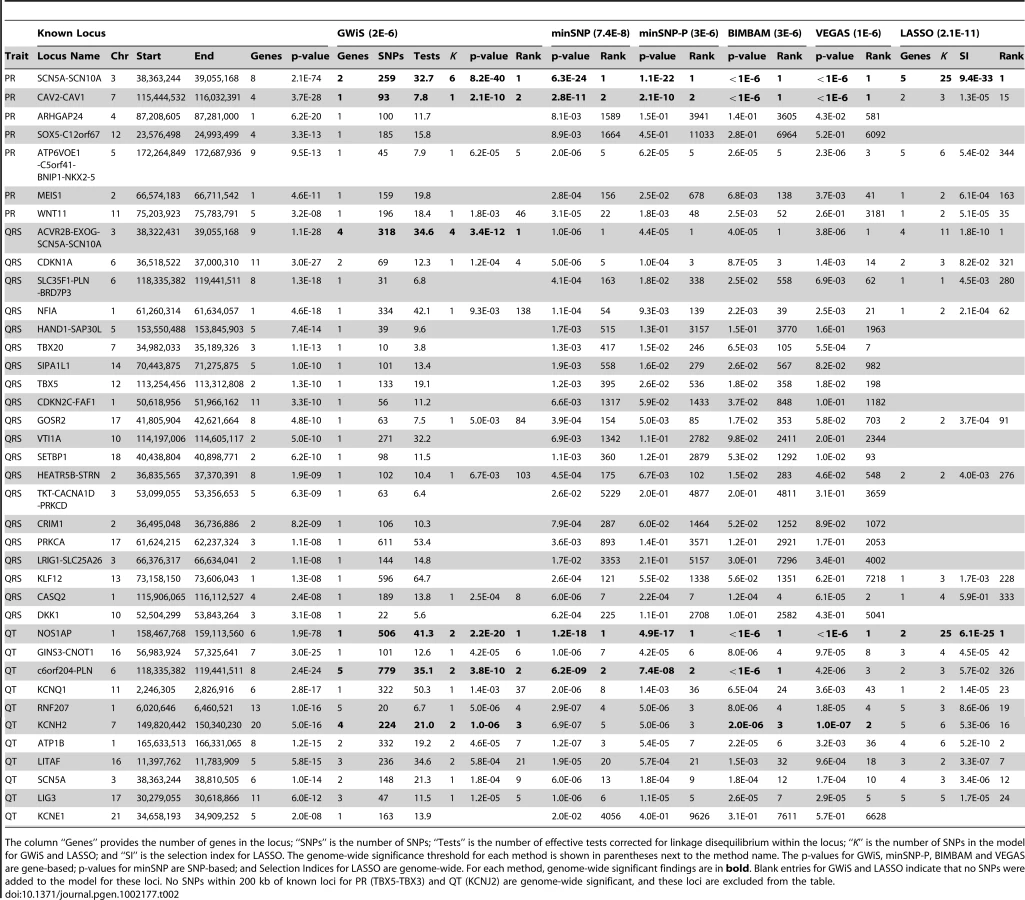
GWiS out-performed all other methods in the comparison (Figure 3 and Table 2). GWiS identifies 6 of 38 known genes or loci as genome-wide significant. In contrast, BIMBAM identifies 5 known positives; minSNP, minSNP-P and VEGAS identify 4; and LASSO identifies 2. Loci identified by the other methods are all subsets of the 6 found by GWiS. None of the methods produced any false positives at genome-wide significance.

Due to the limited size of the ARIC cohort relative to the studies that generated the known positives, no method was expected to find all 38 known loci to be genome-wide significant. Nevertheless, known positives should still rank high among the top predictions of each method, assessed by the ranks of the known positives at 40% recall (Figure S3). We found that GWiS, minSNP, minSNP-P, BIMBAM, and VEGAS were equally effective in ranking known positives (Mann-Whitney rank sum p-values for any pairwise comparison). LASSO performed below the other methods (p-value for a pairwise comparison of LASSO to any other method). Top associations (up to 100 false positives) from each method are provided for PR interval, QRS interval, and QT interval (Tables S3, S4, S5).
While our conclusions are based on cardiovascular phenotypes, the results suggest that GWiS will have an advantage when causal genes have multiple effects. When an association is sufficiently strong to be found by a univariate test, GWiS is generally able to identify it. Beyond these association, GWiS is also able to detect genes that are genome-wide significant, but where no single effect is large enough to be significant by univariate tests. The association of QRS interval with SCN5A-SCN10A is a striking example: 4 independent effects are found by GWiS (p-value = ) but the association is not genome-wide significant by univariate methods (p-value = for minSNP-P) (Figure 4). A common follow-up strategy for single-SNP methods is to search for secondary associations in the same locus as a strong primary association. These results for ARIC together with results above for simulated data (Figure 2) demonstrate that GWiS performs this task well. While this feature is present in previous follow-up methods for candidate loci [11], [33], [34], it is absent from methods generally used for primary analysis of GWAS data.

Of the 38 known positives, 20 have GWiS models with at least one SNP (regardless of genome-wide significance), and 7 of these are predicted to have multiple independent effects (Figure 5). These results suggest that the genetic architecture of ECG traits supports the hypothesis underlying GWiS. Moreover, for QT interval where the power is greatest to identify known positives (the ARIC sample size is 50% of the GWAS discovery cohorts), 5 of the 10 loci identified by GWiS are predicted to have multiple independent effects.

Discussion
In summary, we describe a new method for gene-based tests of association. By gathering multiple independent effects into a single test, GWiS has greater power than conventional tests to identify genes with multiple causal variants. GWiS also retains power for low-frequency minor alleles that are increasingly important for personal genetics, a feature not shared by other multi-SNP tests.
Furthermore, GWiS provides an accurate, conservative estimate for the number of independent effects within a gene or region. Currently there are no standard criteria for establishing the genome-wide significance of a weak second association in a gene whose strongest effect is genome-wide significant. While the number of effects can be provided by existing Bayesian methods [34], their computational expense has limited their applicability to candidate regions, and they are not routinely used. By providing a computationally efficient alternative to existing methods, GWiS provides a new capability to estimate the number of effects as part of primary GWAS data analysis. Demonstrated effectiveness on real data may lead to more widespread use of this type of analysis. Applied to cardiovascular phenotypes relevant to sudden cardiac death and atrial fibrillation, GWiS indicates that 35 to 50% of all known loci contain multiple independent genetic effects.
The test we describe includes a prior on models designed to be unaffected by SNP density, in particular by the number of SNPs that are well-correlated with a causal variant. The priors on regression parameters are essentially uniform, with the benefit of eliminating any user-adjustable parameters. A theoretical drawback is that the priors are improper [35], [36]. Theoretical concerns are mitigated, however, because improper priors pose no challenge for model selection, and our permutation procedure ensures uniform p-values under the null.
Bayesian methods can be computationally expensive. GWiS minimizes computation by evaluating only the locally optimal models of increasing size in a greedy forward search. This appears to be an approximation compared to previous Bayesian methods that sum over all models. Previous Bayesian methods entail their own approximations, however, because the search space must either be truncated at 1 or 2 SNPs, heavily pruned, or lightly sampled using Monte Carlo. Our results demonstrate that the approximations used by GWiS provide greater computational efficiency than approximations used in previous Bayesian frameworks, with no loss of statistical power. GWiS currently calculates p-values, rather than Bayesian evidence provided by other Bayesian methods. If Bayesian evidence is desired, an intriguing alternative to Bayesian post-processing of candidate loci might be to use the Bayes Factor from the most likely alternative model identified by GWiS as a proxy for the sum over all alternatives to the null model. This may be an accurate approximation because, in practice, the Bayes Factor for the most likely model from GWiS dominates all other Bayes Factors in the sum.
The GWiS framework, using gene annotations to structure Bayesian model selection, may be applied to case-control data by encoding phenotypes as 1 (case) versus 0 (control), a reasonable approach when effects are small. More fundamental extensions to logistic regression, Transmission Disequilibrium Tests (TDTs), and other tests and designs should be possible and may yield further improvements. Moreover, similar gene-based structured searches can be applied to genetic models to include explicit interaction terms [14]. The Bayesian format also permits incorporation of prior information about the possible functional effects of SNPs [37], [38], and disease linkage [39], [40]. Finally, the gene-based p-values provide a natural entry to gene annotations and pathway-based gene set enrichment analysis [41]–[43].
Materials and Methods
Ethics statement
This research involves only the study of existing data with information recorded in such a manner that the subjects cannot be identified directly or through identifiers linked to the subjects.
Known positives
Known positive associations are taken from published genome-wide significant SNP associations (p-value ) [1], [2], [4], [5]. Genes within 200 kb of any genome-wide significant SNP are scored as known positives. Finally, genes within 200 kb that are both positive are merged into a single known positive locus to avoid over-counting.
Study cohort
The ARIC study includes 15,792 men and women from four communities in the US (Jackson, Mississippi; Forsyth County, North Carolina; Washington County, Maryland; suburbs of Minneapolis, Minnesota) enrolled in 1987-89 and prospectively followed [44]. ECGs were recorded using MAC PC ECG machines (Marquette Electronics, Milwaukee, Wisconsin) and initially processed by the Dalhousie ECG program in a central laboratory at the EPICORE Center (University of Alberta, Edmonton, Alberta, Canada) but during later phases of the study using the GE Marquette 12-SL program (2001 version) (GE Marquette, Milwaukee, Wisconsin) at the EPICARE Center (Wake Forest University, Winston-Salem, North Carolina). All ECGs were visually inspected for technical errors and inadequate quality. Genotype data sets were cleaned initially by discarding SNPs with Hardy-Weinberg equilibrium violations at p , minor allele frequencies , or call rates . Imputation with HapMap CEU reference panel version 22 was then performed, and all imputed SNPs were retained for analysis, included imputed SNPs with minor-allele frequencies as low as 0.001. These cleaned data sets contributed to the meta-analysis to yield the known positives, and full descriptions of phenotype and sample data cleaning are available elsewhere [1], [2], [4]. Regional association plots were generated using a modified version of “make.fancy.locus.plot” [45].
Conventional multiple regression
The phenotype vector Y for N individuals is an vector of trait values. The genotype matrix X has N rows and P columns, one for each of P genotyped markers assumed to be biallelic SNPs. For simplicity, the vector Y and each column of X are standardized to have zero mean. A standard regression model estimates the phenotype vector as , where b is a vector of regression coefficients and e is a vector of residuals assumed to be independent and normally distributed with mean 0 and variance . The log probability of the phenotypes given these parameters is(1)
The maximum likelihood estimators (MLEs) are and , where denotes the transpose of . The total sum-of-squares (SST) is , and the sum-of-squares of the model (SSM) is . The sum-of-squares of the errors or residuals (SSE) is(2)
A conventional multiple regression approach uses the F-statistic to decide whether adding a new SNP improves the model significantly,(3)for a model with K SNPs, distributed as under the null. This approach fails, however, when the best SNPs are selected from the much larger number of M total SNPs, because the statistic does not account for the selection process.
Bayesian model selection
A model M is defined as the subset of SNPs in a gene with P total SNPs that are permitted to have non-zero regression coefficients. For each gene, GWiS attempts to find the subset that maximizes the model probability , where each of the P columns of X corresponds to a SNP assigned to the gene. In the absence of association, the null model with = 0 usually maximizes the probability, indicating no association. When a model with maximizes the probability, an association is possible, and permutation tests provide a p-value. According to Bayes rule,(4)
The factor is model-independent and can be ignored.
The prior probability of the model, , assumes that each of the P SNPs within the gene has an identical probability of being associated with the trait. This probability, denoted f, is unknown, and is integrated out with a uniform prior. The prior is also designed to make the model probability insensitive to SNP density: it should be unaffected if an existing SNP is replicated to create a new SNP marker with identical genotypes. We do this by replacing the number of SNPs within a gene with an effective number of tests, , calculated from the local LD within a gene. Correlations between SNPs make the effective number of tests smaller than the number of SNPs. The model prior based on the effective number of tests is(5)or for integer values. As the effective number of tests, , whose calculation is described below, is generally non-integer, we use the standard Beta function rather than factorials.
The remaining factor in Eq. 4 is(6)
The integration limits and prefactor ensure normalization. We assume that these limits are sufficiently large to permit a steepest descents approximation as in Schwarzian BIC model selection [15]. First, assuming that the genotypes are centered, the genotype covariance matrix is , where indicates matrix transpose as before, and diagonal elements for SNP with allele frequency . Provided that is much greater than each component of , the integral over is approximately(7)where the sum-squared-error SSE is . Provided that the limit is much greater than the maximum likelihood value , the integral over can be approximated as(8)where is the standard Gamma function. To avoid the cost of Gamma function evaluations, we instead use the steepest descents approximation,(9)
The log-likelihood is then(10)
As in the BIC approximation, we retain only terms that depend on the model and are of order or greater. Thus we replace by , and . For historical reasons, we also included a factor of in the prior for model size, to yield the asymptotic approximation(11)
The strategy of GWiS is therefore to find the model that maximizes the objective function(12)
The terms involving provide a Bayesian penalty for model performance, but also make this an NP-hard optimization problem. We have adopted two efficient deterministic heuristics for approximate optimization. First is a greedy forward search, essentially Bayesian regularized forward regression, in which the SNP giving the maximal increase to the model likelihood is added to the model sequentially until all remaining SNPs decrease the likelihood. The second is a similar heuristic, except that the initial model searches through all subsets of 2 SNPs or 3 SNPs. We adopted this subset search to permit the possibility that all = 1 models are worse than the = 0 null, whereas a more complex model with or 3 has higher score. In practice, all associations identified by subset selection were also identified by greedy forward search. We therefore used the greedy forward search for computational efficiency.
GWiS is designed to select a single model for each gene. An alternative related approach would be to test for the posterior probability of the null model, , against all other models, + + + , using our model selection procedure either to choose the locally best model of each size or to include multiple models (which could suffer from a systematic bias favoring SNPs in large LD blocks). This is in fact the strategy of BIMBAM, which attempts to systematically evaluate all terms up to a given model size. Unfortunately, the number of terms increases exponentially fast with model size, and the brute-force approach does not scale to genome-wide applications. Monte Carlo searches over models have also been difficult to apply genome-wide. Our work suggests that approximations that limit the search for fixed model size can be accurate, and further that the probabilities of models that are too large are expected to decrease exponentially fast, permitting the sum to be pruned and truncated. We have observed in practice that the model with the most likely value of dominates the sum, and similarly for BIMBAM that the single SNP with the best Bayes Factor dominates the sum-of-Bayes-Factors test statistic. These results suggest that the results of a more computationally expensive sum over all models would be largely consistent with the results of GWiS method. Furthermore, the Bayes Factor for the most likely model could provide a proxy for the Bayesian evidence.
Effective number of tests
The effective number of tests is an established concept in GWAS to provide a multiple-testing correction for correlated markers. While the exact correction can be established by permutation tests, faster approximate methods can perform well [46]–[49]. While we use a fast procedure, a final permutation test ensures that p-values are uniform under the null.
The method we adopt is based on multiple linear regression of SNPs on SNPs. The genotype vector for each SNP i is standardized to have zero mean. Correlations between all pairs of SNPs i and j are initialized as . Each SNPs weight is initialized to 1, and the number of effective tests T is initialized to 0. The SNP i with maximum weight is identified, and the following updates are executed:(13)
This process continues until all weights are equal to zero. When SNPs with maximum weight are tied (as occurs for the first SNP processed), the SNP with lowest genomic coordinate is selected to ensure reproducibility; we have ensured that this method is robust to other methods for breaking ties, including random selection. For simplicity, the correlations are not updated (the update rule would be ), which may lead to an overestimate for T. Model selection may therefore have a conservative bias. The p-values are not affected, however, because they are calculated by permutation tests as described below.
The effective number of tests implies a trivial renormalization of the model prior, (Eq. 5), that does not affect the test statistic. Letting be the total number of markers, be the effective number tests, and be the size of the model, our prior gives each model of size the weight . If and are identical, there are models of this size, and the total weight of all models of size is . Since can range from 0 to , the sum is normalized. But when is larger than , the sum of all models of size is , which is . The sum from to is therefore . A normalization of 1 can be recovered by including an overall normalization factor, . The explicit prior for models of size is , which is normalized to 1. Since is model-independent, it does not contribute to the test statistic.
P-values and genome-wide significance
We use two stages of permutation tests: the first stage converts the GWiS test statistic into a p-value that is uniform under the null; the second stage establishes the p-value threshold for genome-wide significance.
The first stage is conducted gene-by-gene. We permute the trait array using the Fisher-Yates shuffle algorithm [50], [51] and use the permuted trait to calculate the test statistics using the same procedure as for the original trait. Specifically, the model size is optimized independently for each permutation, with most permutations correctly choosing = 0. For S successes (log-likelihoods greater than or equal to the unpermuted phenotype data) out of Q permutations, the empirical p-value is S/Q. To save computation, permutations are ended when . Furthermore, once a finding is genome-wide significant, there is no practical need for additional permutations. For gene-based tests (GWiS, minSNP-P, BIMBAM, and VEGAS), the p-value for genome-wide significance depends on the number of genes tested (rather than the number of SNPs), for humans. We therefore also terminate permutations after Q = 1 million trials, regardless of S. In these cases, for purposes of ranking, a parametric p-value is estimated for GWiS as(14)
The first factor is the parametric p-value for the F statistic from the MLE fit, and the second term is the combinatorial factor for the number of possible models of the same size.
While these p-values are uniform under the null, the threshold for genome-wide significance requires a second set of permutations. To establish genome-wide significance thresholds, in the second stage we permuted the ARIC phenotype for each trait 100 times, ran GWiS for the permuted phenotypes on the entire genome, and recorded the best genome-wide p-value from each of the 100 permutations. We then combined the results from each trait to obtain an empirical distribution of the best genome-wide p-value under the null. We then estimated the p = 0.05 genome-wide significance threshold as the 15th best p-value of the 300. This procedure was performed for GWiS, minSNP, minSNP-P, LASSO, and VEGAS to obtain genome-wide significance thresholds for each. Since minSNP-P and BIMBAM are both uniform under the null, we used the genome-wide significance threshold calculated for minSNP-P, , for BIMBAM to avoid additional computional cost (Table S2). The threshold for GWiS is more stringent, , presumably because of the locus merging procedure described below. Changes in the genome-wide significance thresholds of up to 50% would not affect any of the reported results.
Hierarchical analysis of genetic loci
In a region with a strong association and LD, GWiS can generate significant p-values for multiple genes in a region. A hierarchical version of GWiS is used to distinguish between two possibilities. First, through LD, a strong association in one gene may cause a weaker association signal in a second gene. In this case, only the strong association should be reported. Second, the causal variant may not be localized in a single gene; for example, the best SNP tags are assigned to multiple genes. In this case, the individual genes should be merged into a single associated locus. The hierarchical procedure is as follows.
-
Identify all genes with GWiS , and use transitive clustering to merge into a locus all genes whose transcript boundaries are within 200 kb.
-
Run GWiS on the merged locus (including a recalculation of the number of effective tests within the locus) and identify the SNPs selected by the GWiS model. If genes at either end of the locus have no GWiS SNPs, trim these genes from the locus. Repeat this step until no more trimming is possible. If only a single gene remains, accept it with its original p-value as the only association in the region. Otherwise, proceed to step 3.
-
Use a permutation test to calculate the p-value for the merged locus from step 2. Assign it a p-value equal to the minimum of the p-values from the individual genes, and the p-value from its own permutation. Regardless of the p-value used, retain the entire trimmed region as an associated locus.
The trimming in step 2 handles the first possibility, a strong association in one gene that causes a weaker association in a neighbor. The rationale for accepting the smallest p-value in step 3 is the case of a single SNP assigned to multiple genes. The merged region will have a less significant p-value than any single gene, and it does not seem reasonable to incur such a drastic penalty for gene overlap.
Univariate tests: minSNP and minSNP-P
For these tests, SNPs are assigned to gene regions as before. The p-value for each SNP is then calculated using the F-statistic as the test statistic, with empirical p-values from permutation to ensure correct p-values for SNPs with low minor allele frequencies. The minSNP method assigns a gene the p-value of its best SNP. Selection of the best p-value out of many leads to non-uniform p-values under the null. It is standard to reduce this bias by scaling p-values by a Bonferroni correction based on the number of SNPs or number of estimated tests. Instead, we perform gene-by-gene permutation tests using the best F statistic for SNPs within the gene as the test statistic. As with GWiS, if 1 million permutations do not lead to one success, the association is clearly genome-wide significant and we use the Bonferroni-corrected p-value for ranking purposes.
BIMBAM
The Bayesian Imputation-based Association Mapping (BIMBAM) is a Bayesian gene-based method [10]. BIMBAM calculates the Bayes Factor for a model and then averages the Bayes Factors for all models within a gene to obtain a test statistic. Because 1-SNP models were found to have as much power as 2-SNP models, and because 2-SNP models are not computationally feasible for genome-wide analysis, BIMBAM by default restricts its sum to all 1-SNP models within a gene [10]. The Bayes Factor for a single SNP is(15)
The design matrix has first column s and second column equal to the dosages of SNP in the individuals; is the phenotypic mean; ; the matrix is diagonal with diagonal terms ; and contains the regression coefficients . We used the recommended value relative to the phenotypic standard deviation. The test statistic for a gene with SNPs is . As with other methods, we used gene-by-gene permutations to convert this statistic into a p-value that is uniform under the null. Up to 1 million permutations were used, stopping after 10 successes.
The sufficient statistics used by BIMBAM are identical to minSNP and minSNP-P, yet we found that the runtime of the public implementation was much slower, taking 270 sec for 1000 permutations of a gene with 135 SNPs across 8000 individuals. By improving memory management and optimizing computations, we improved the timing to 14 sec per 1000 permutations, a 19-fold speed-up. This implementation is included in our Supplementary Materials.
VEGAS
The Versatile Gene-Based Test for Genome-wide Association (VEGAS) [25] is a recently proposed method that considers the SNPs within a gene as candidates for association study. VEGAS assigns SNPs to each of the autosomal genes using the UCSC genome browser hg18 assembly. The gene boundaries are defined as of the and UTRs. Single SNP p-values are used to compute a gene-based test statistic for each gene and significance of each gene is evaluated using simulations from a multivariate normal distribution with mean 0 and covariance matrix being the pairwise LD values between the SNPs from HapMap Phase 2. As a result the method avoids permutations in calculating per gene p-values, although permutations are required to obtain the genome-wide significance threshold.
LASSO regression
LASSO regression is a recent method for combined model selection and parameter estimation that maps L1 regularized regression onto a computationally tractable quadratic optimization problem [26]–[28]. Applications to GWAS are attractive because it is possible to perform model selection on an entire chromosome. We therefore implemented a recent LASSO procedure developed specifically for GWAS [29].
To reduce computational cost, univariate p-values are estimated from parametric tests, and gene-based SNPs with are retained (we have confirmed that this computational constraint does not lose any known positive associations). Incremental model selection was performed by Least Angle Regression [27] using the R lars package [52]. The LASSO parameter was determined using 5-fold cross validation. All genes with at least one SNP selected were identified, and selected genes overlapping other selected genes (including flanking regions) were merged into single loci.
As suggested previously, we used the Selection Index to rank genes and as the test statistic for a permutation p-value [29]. To obtain the Selection Index, the MLE log-likelihood is calculated for the full model and for a reduced model with a subset of SNPs removed. Twice the log-likelihood difference is interpreted as a statistic, and the Selection Index is defined as the corresponding p-value for a distribution with the number of removed SNPs as the degrees of freedom. Due to the LASSO model selection procedure, the Selection Index is not distributed as a under the null, and permutation tests are used to establish genome-wide significance levels.
Simulations: power
For each true model size of to 8, we performed a series of simulations by picking 1000 genes from chromosome 1 randomly with replacement, using genotype data from the ARIC population of approximately 8000 individuals. For each gene, we selected “causal” SNPs that have from regression with other “causal” SNPs within the gene. A gene had to have at least SNPs to be picked for models of size to ensure enough remaining SNPs after the removal of the causal SNPs to permit a model of the true size.
We attempted to distribute the total population variance explained, , equally across the SNPs. The covariance matrix for the SNPs calculated from the population is denoted , with understood to be . The coefficient for SNP in the model was set to(16)which ensures that . The phenotype for an individual with genotype row-vector was then calculated as , with again the population average of and drawn from a standard normal distribution.
The power was calculated as (number of genes that are genome-wide significant)/1000, and the error of the estimate was calculated using 95% exact binomial confidence intervals. The p-value thresholds were taken directly from genome-wide permutations (Table 2).
Simulations: model size
Phenotypes that were used to estimate the model size were generated by assigning each “causal” SNP the same power of 0.1 and 0.8. The population variance explained for each SNP was calculated as , in which is the quantile of the standard normal for upper-tail cumulative probability of , and is the quantile for lower-tail probability power. We chose to be , the commonly used genome-wide significance threshold for univariate tests. The effect of SNP is then , in which is the genotype covariance matrix. The simulated phenotypes are then , with drawn from a standard normal distribution. In this test we control for the variance explained by the SNP, not by the gene, and therefore do not rescale the regression coefficients to account for LD. For each ranging from 0 to 10, we repeated these steps using ARIC genotype data for 100 genes chosen at random from chromosome 1.
Only GWiS and LASSO give model size estimates. GWiS directly reports the model size as the number of independent effects within a gene and LASSO reports the model size as the number of selected SNPs within a gene. We ran both methods using the simulated data with LD. We also tested both scenarios when the causal SNPs were kept or removed from gene.
Performance evaluation
Gene associations were scored as true positives if the gene (or merged locus) overlapped with a known association, and as false positives if no overlap exists. Only the first hit to a known association spanning several genes was counted.
The primary evaluation criterion is the ability to identify known positive associations at genome-wide significance. The genome-wide significance threshold was determined separately for each method (see above), and no method gave any false positives at its appropriate threshold.
A secondary criterion was the ability to enrich highly ranked loci for known associations, regardless of genome-wide significance. This criterion was assessed through precision-recall curves, with precision = TP/(TP+FP), recall = TP/(TP+FN), and true positives (TP), false positives (FP), and false negatives (FN) defined as a function of the number of predictions considered.
Small differences in precision and recall may not be statistically significant. To estimate statistical significance, we performed a Mann-Whitney rank sum test for the ranks of the known associations at 40% recall for GWiS, minSNP, minSNP-P, and LASSO.
Implementation
GWiS runs efficiently in memory and CPU time, roughly equivalent to other genome-wide tests that require permutations (Table 3). Computational times are greater for real data because real associations with small p-values require more permutations. LASSO required far less computational resources, but also pre-filtered the SNPs and had the worst performance. Genome-wide studies can be finished within around 100 hours. Low memory requirements allow GWiS to run in parallel on multiple CPUs. The GWiS source code implementing GWiS, minSNP, minSNP-P, and BIMBAM is available under an open source GNU General Public License as Supplementary Material, also from the authors' website (www.baderzone.org), and is being incorporated into PLINK [31].

Supporting Information
Zdroje
1. PfeuferAvan NoordCMarcianteKDArkingDELarsonMG 2010 Genome-wide association study of pr interval. Nat Genet
2. SotoodehniaNIsaacsAde BakkerPIWDrrMNewton-ChehC 2010 Common variants in 22 loci are associated with qrs duration and cardiac ventricular conduction. Nat Genet
3. ArkingDEPfeuferAPostWKaoWHNewton-ChehC 2006 A common genetic variant in the nos1 regulator nos1ap modulates cardiac repolarization. Nat Genet 38 644 51
4. PfeuferASannaSArkingDEMullerMGatevaV 2009 Common variants at ten loci modulate the qt interval duration in the qtscd study. Nat Genet 41 407 14
5. Newton-ChehCEijgelsheimMRiceKMde BakkerPIYinX 2009 Common variants at ten loci inuence qt interval duration in the qtgen study. Nat Genet 41 399 406
6. NealeBMShamPC 2004 The future of association studies: gene-based analysis and replication. Am J Hum Genet 75 353 62
7. BallardDHChoJZhaoH 2009 Comparisons of multi-marker association methods to detect association between a candidate region and disease. Genet Epidemiol
8. ChapmanJWhittakerJ 2008 Analysis of multiple snps in a candidate gene or region. Genet Epidemiol 32 560 6
9. WilleAHohJOttJ 2003 Sum statistics for the joint detection of multiple disease loci in case-control association studies with snp markers. Genet Epidemiol 25 350 9
10. ServinBStephensM 2007 Imputation-based analysis of association studies: candidate regions and quantitative traits. PLoS Genet 3 e114 doi:10.1371/journal.pgen.0030114
11. FridleyBL 2009 Bayesian variable and model selection methods for genetic association studies. Genet Epidemiol 33 27 37
12. GeorgeEIMcCullochRE 1993 Variable selection via gibbs sampling. Journal of the American Statistical Association 88 881 889
13. BallRD 2001 Bayesian methods for quantitative trait loci mapping based on model selection: approximate analysis using the bayesian information criterion. Genetics 159 1351 64
14. BogdanMGhoshJKDoergeRW 2004 Modifying the schwarz bayesian information criterion to locate multiple interacting quantitative trait loci. Genetics 167 989 99
15. SchwarzG 1978 Estimating the dimension of a model. The Annals of Statistics 6 461 464
16. ChengSKeyesMJLarsonMGMcCabeELNewton-ChehC 2009 Long-term outcomes in individuals with prolonged pr interval or first-degree atrioventricular block. JAMA 301 2571 7
17. VrtovecBDelgadoRZewailAThomasCDRichartzBM 2003 Prolonged qtc interval and high b-type natriuretic peptide levels together predict mortality in patients with advanced heart failure. Circulation 107 1764 9
18. SchoutenEGDekkerJMMeppelinkPKokFJVandenbrouckeJP 1991 Qt interval prolongation predicts cardiovascular mortality in an apparently healthy population. Circulation 84 1516 23
19. GrigioniFCarinciVBorianiGBracchettiGPotenaL 2002 Accelerated qrs widening as an independent predictor of cardiac death or of the need for heart transplantation in patients with congestive heart failure. J Heart Lung Transplant 21 899 902
20. TurriniPCorradoDBassoCNavaABauceB 2001 Dispersion of ventricular depolarization-repolarization: a noninvasive marker for risk stratification in arrhythmogenic right ventricular cardiomyopathy. Circulation 103 3075 80
21. SayersEWBarrettTBensonDABryantSHCaneseK 2009 Database resources of the national center for biotechnology information. Nucleic Acids Res 37 D5 15
22. DixonALLiangLMoffattMFChenWHeathS 2007 A genome-wide association study of global gene expression. Nat Genet 39 1202 7
23. StrangerBENicaACForrestMSDimasABirdCP 2007 Population genomics of human gene expression. Nat Genet 39 1217 24
24. VeyrierasJBKudaravalliSKimSYDermitzakisETGiladY 2008 High-resolution mapping of expression-qtls yields insight into human gene regulation. PLoS Genet 4 e1000214 doi:10.1371/journal.pgen.1000214
25. LiuJZMcRaeAFNyholtDRMedlandSEWrayNR 2010 A versatile gene-based test for genome-wide association studies. Am J Hum Genet 87 139 145
26. TibshiraniR 1996 Regression shrinkage and selection via the lasso. J Roy Statist Soc Ser B 58 267 288
27. EfronBHastieTJohnstoneITibshiraniR 2002 Least angle regression
28. WuTLangeK 2008 Coordinate descent algorithms for lasso penalized regression. Annals of Applied Statistics 2 224 244
29. WuTTChenYFHastieTSobelELangeK 2009 Genome-wide association analysis by lasso penalized logistic regression. Bioinformatics 25 714 21
30. WolpertDHMacreadyWG 1997 No free lunch theorems for optimization. IEEE transactions on evolutionary
31. PurcellSNealeBTodd-BrownKThomasLFerreiraMA 2007 Plink: a tool set for whole-genome association and population-based linkage analyses. Am J Hum Genet 81 559 75
32. ChurchillGADoergeRW 1994 Empirical threshold values for quantitative trait mapping. Genetics 138 963 71
33. VerzilliCShahTCasasJPChapmanJSandhuM 2008 Bayesian meta-analysis of genetic association studies with different sets of markers. American journal of human genetics 82 859 872
34. StephensMBaldingDJ 2009 Bayesian statistical methods for genetic association studies. Nature Reviews Genetics 10 681 690
35. LindleyD 1957 A statistical paradox. Biometrika 44 187
36. BartlettM 1957 A comment on dv lindley's statistical paradox. Biometrika 44 533
37. ClineMKarchinR 2010 Using bioinformatics to predict the functional impact of snvs. Bioinformatics (Oxford, England)
38. AdzhubeiIASchmidtSPeshkinLRamenskyVEGerasimovaA 2010 A method and server for predicting damaging missense mutations. Nat Methods 7 248 9
39. McKusickVA 2007 Mendelian inheritance in man and its online version, omim. Am J Hum Genet 80 588 604
40. FridleyBLSerieDJenkinsGWhiteKBamletW 2010 Bayesian mixture models for the incorporation of prior knowledge to inform genetic association studies. Genet Epidemiol 34 418 26
41. SubramanianATamayoPMoothaVKMukherjeeSEbertBL 2005 Gene set enrichment analysis: a knowledge-based approach for interpreting genome-wide expression profiles. Proceedings of the National Academy of Sciences of the United States of America 102 15545 50
42. WangKLiMBucanM 2007 Pathway-based approaches for analysis of genomewide association studies. American journal of human genetics 81
43. HoldenMDengSWojnowskiLKulleB 2008 Gsea-snp: applying gene set enrichment analysis to snp data from genome-wide association studies. Bioinformatics 24 2784 5
44. The ARIC investigators 1989 The atherosclerosis risk in communities (aric) study: design and objectives. Am J Epidemiol 129 687 702
45. SaxenaRVoightBF Diabetes Genetics Initiative of Broad Institute of Harvard and MIT, Lund University, Novartis Institutes of BioMedical Research 2007 Genome-wide association analysis identifies loci for type 2 diabetes and triglyceride levels. Science 316 1331 1336
46. CheverudJM 2001 A simple correction for multiple comparisons in interval mapping genome scans. Heredity 87 52 8
47. NyholtDR 2004 A simple correction for multiple testing for single-nucleotide polymorphisms in linkage disequilibrium with each other. American journal of human genetics 74 765 9
48. LiJJiL 2005 Adjusting multiple testing in multilocus analyses using the eigenvalues of a correlation matrix. Heredity 95 221 7
49. GalweyNW 2009 A new measure of the effective number of tests, a practical tool for comparing families of non-independent significance tests. Genet Epidemiol 33 559 68
50. FisherRAYatesF 1938 Statistical tables for biological, agricultural and medical research. London [etc.] Oliver and Boyd. 39000863 by R.A. Fisher … and F. Yates … 29 cm. "References": 23
51. KnuthDE 1997 The art of computer programming. Reading, Mass: Addison-Wesley, 3rd edition 97002147 Donald E. Knuth. ill. ; 24 cm. Includes indexes. v. 1. Fundamental algorithms – v. 2. Seminumerical algorithms – v. 3. Sorting and searching
52. HastieTEfronB 2009 lars: Least angle regression, lasso and forward stagewise
Štítky
Genetika Reprodukční medicínaČlánek vyšel v časopise
PLOS Genetics
2011 Číslo 7
Nejčtenější v tomto čísle
- A Rice Plastidial Nucleotide Sugar Epimerase Is Involved in Galactolipid Biosynthesis and Improves Photosynthetic Efficiency
- Genome-Wide Association Study Identifies Novel Restless Legs Syndrome Susceptibility Loci on 2p14 and 16q12.1
- Loss of the BMP Antagonist, SMOC-1, Causes Ophthalmo-Acromelic (Waardenburg Anophthalmia) Syndrome in Humans and Mice
- Gene-Based Tests of Association